Capital Market Assumptions 2024

"Our long-term return expectations for capital markets serve as key inputs into our strategic asset allocation process for multi-asset portfolios and provide context for shorter-term forecasting.

Foreword

Each year, the Voya Multi-Asset Strategies and Solutions team formulates capital market forecasts for the coming decade. This exercise is an opportunity for us to step back from the day-to-day noise within the markets and consider longer-term trends in economic and financial factors that are likely to drive asset class return and risk. We rely on these assumptions to set our strategic asset allocations for our multi-asset portfolios.

In conducting our analysis, we look at numerous macroeconomic and financial data series to generate our forecasts. For example, how do labor force participation rate expectations impact potential GDP? Are profit margins likely to mean-revert? What are the long-run trends in productivity?

"The next decade will likely be characterized by returns below historical averages across all major asset classes.

To avoid the pitfalls of single-point estimates, we incorporate an alternative macroeconomic scenario into our forecasts. We produce blended estimates for our base and alternative scenarios that prevent us from becoming too upbeat or downbeat in our forecasting techniques or extrapolating from the recent past. Our uncertainty measures of our forecasts similarly blend two estimates of risk, leading to more resilient portfolios. For any fiduciary or person managing assets with a long investment time horizon, this exercise combines both judgment and quantitative inputs, which are reflected in the forecasts.

Given higher valuations and lower risk premiums in equity markets, our analysis for the 2024–2033 period paints a picture of relatively low expected returns for equities. In contrast, our outlook for bonds has improved, owing to higher starting bond yields compared with the depressed levels of 2022. Return forecasts are generally above inflation and, if our expectations prove broadly correct, asset allocators will find numerous opportunities to generate alpha across and within asset classes after 2022’s losses and high asset class correlations.

We hope this report provides a helpful reference for your own decision-making process, and we wish you a successful 2024.

Summary of findings

Our Capital Market Assumptions (CMA) 2024 report details our research on asset class returns, standard deviations of returns and correlations over the 10-year horizon from 2024 through 2033. These estimates represent key inputs into strategic asset allocation decisions for our multi-asset portfolios and provide context for shorter-term macroeconomic and financial forecasting.

Our forecasts were informed by historically low potential gross domestic product (GDP) growth, reduced labor supply and elevated inflation. To avoid using a single-point-estimate forecast, we incorporate an alternative scenario, which can have slightly better or worse macro inputs. Similar to last year, this year’s alternative scenario was based on marginally higher productivity and a lower terminal federal funds rate.

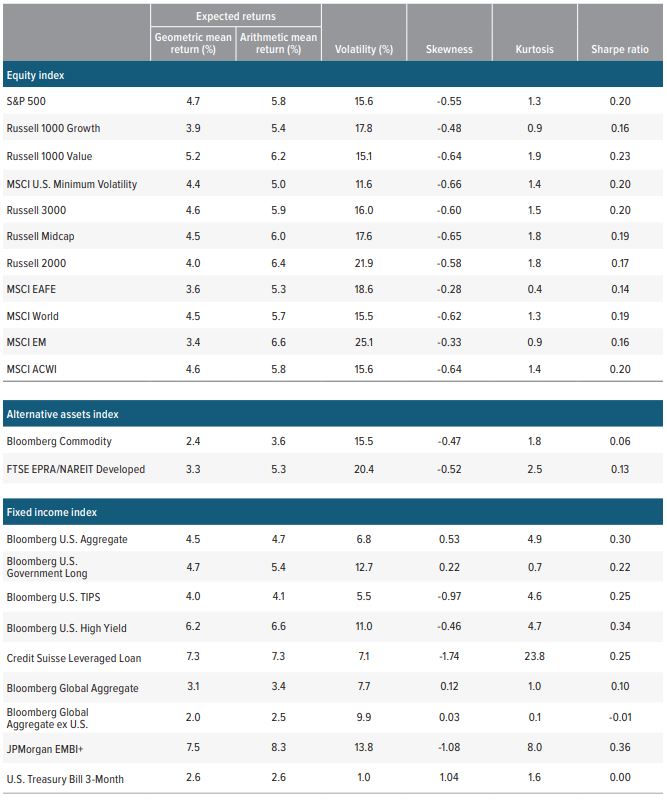
"Compared to last year’s projections, our 2024–2033 forecast calls for similar equity returns (5.8% for the S&P 500) and higher bond returns (4.7% for the U.S. Agg).

Some key results of our analysis:

• The next decade will likely be characterized by returns below historical averages across all major asset classes.
• Developed market equities are likely to deliver mid-single digit returns, with U.S. markets higher than most comparable non-U.S. ones.
• Emerging market equities should outperform developed markets, albeit with higher expected volatility given a more uncertain path to growth.
• Bond return assumptions have increased from last year but remain in the low single digits. These projections assume that moves in bond term premiums and real interest rates will cap the upside return potential of fixed income assets.

Ten-year forecast: Low growth persists globally, but the U.S. offers upside potential

Our forecast models an explicit process of convergence toward a steady-state equilibrium for global economies and financial markets through 2033. In our modeling process, we worked with the economic consulting group at S&P Global, which provided quantitative support for our macro inputs.¹

Cyclical fluctuations are an inevitable aspect of market economies, and we recognize that the steady-state equilibrium incorporated as the terminal point of our 10-year forecast is unlikely to be fully attained under real world conditions. Nonetheless, we find that this theoretical construct is useful for anchoring the forecast. As a result, the forecast does not assume a recession or contraction over the 2024–2033 horizon.

Throughout the period covered by our forecast, we believe the U.S. will be constrained by labor force growth but can move to a somewhat higher, sustained growth path than it experienced in the previous business cycle. The key for the U.S. is to exit the current low productivity regime that has constrained the economy.

Productivity growth essentially comes from capital deepening and total factor productivity (TFP). The latter is an unobservable measure taken from the decomposition of real GDP growth—the remainder after accounting for the contributions of capital and labor, called Solow’s residual. This residual could reflect improvements in technology, growth in the effectiveness of labor, strength in property rights and the quality of labor. It also incorporates cultural attitudes, including risk and high levels of confidence in the outlook, which can contribute to a revival in productivity through the TFP channel.

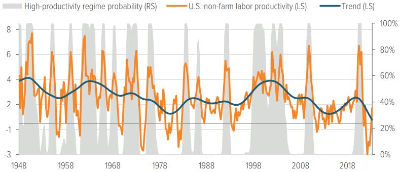
Labor-force productivity growth typically alternates between high- and low-productivity regimes over time. To determine the current regime, we fit productivity data through a Markov model (Exhibit 1). The latest productivity data show that after falling into negative productivity growth in 1Q22, U.S. year-over-year productivity growth turned positive in 2Q23 and continued to rebound to 2.2% in 3Q23. Despite this upward move, the data still signal a low-productivity regime. (Low-productivity regimes, indicated below in the nonshaded chart areas, average 1.0%, while high-productivity regimes, indicated in gray shaded areas, average 3.8%.) A Hodrick-Prescott filter–based decomposition of year-over-year productivity growth into trend and cycle components also shows that the current trend of U.S. productivity growth is close to zero.

Exhibit 1. Productivity growth has decelerated

As of 09/30/23. Source: Voya IM. Non-shaded areas in the chart denote low-productivity regimes

"Over the next decade, the U.S. has greater potential for higher, sustained growth than in the previous business cycle.

As in the past, our 2024 CMA forecast is predicated on a “base” and an “alternative” scenario. We assign a 60% weighting to our base scenario and a 40% weighting to our alternative scenario. The alternative scenario assumes that the U.S. exhibits modest improvement in output per hour, largely the result of TFP gains as the labor share shifts away from brick-and-mortar to more productive firms.

Using these 60/40 blended scenarios, we arrived at our 10-year forecast for U.S. GDP growth of 1.8%. Exhibit 2 shows the 2033 values from this forecast, which are consistent with our estimates of longer-term, steady-state values for key U.S. economic variables.

Exhibit 2. Our 2033 forecast for U.S. economic and financial variables

As of 09/30/23. Source: Voya IM, S&P Global. Forecasts are subject to change.

How we forecast returns

As we mentioned, our process for determining asset class risk and return estimates begins with a top-down forecast of economic growth, using a 60/40 blend of base and alternative scenarios. To develop these forecasts, we leverage S&P Global’s economic modeling capabilities. These two scenarios capture the most important upside and downside risks facing the global economy and markets over the forecast horizon. Furthermore, in response to client demand and following guidance from organizations such as the Task Force on Climate-Related Financial Disclosures (TCFD), we have integrated climate scenarios into our economic forecasts this year, described in Methodological Considerations.

Our base case forecasts 1.6% U.S. GDP growth through 2033, driven by below trend productivity growth and subdued labor force growth. The alternative scenario assumes slightly faster productivity growth, a higher dividend payout ratio and more inflation, assuming the Federal Reserve lets the economy run a little hotter than in the base case. Under these assumptions, returns for risk assets are modestly higher in the alternative scenario than in the base case.

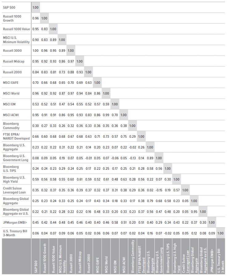
For U.S. stocks, we estimate earnings and dividends for the S&P 500 Index using our blended macroeconomic assumptions. Earnings growth is constrained by the neoclassical assumption that profits as a share of GDP cannot increase without limit but converge to a long-run equilibrium. We then use a dividend discount model to determine fair value for the Index each year during the forecast period. We construct returns for other U.S. equity indexes, including REITs, using a single-index factor model in which beta sensitivities of each asset class with respect to the market portfolio are derived from our forward-looking covariance matrix estimation (Exhibit 3). Beta is, by definition, covariance over variance. (For additional detail, see “Covariance and correlation matrices methodology”.) Each equity asset class return is the sum of the risk-free interest rate and a specific risk premium determined by our estimate of beta sensitivity and market risk premium forecasts (Exhibit 4).

For U.S. bonds, we use the blended scenario interest rate expectations to calculate expected returns for various durations. We model expected bond returns as the sum of current yield and a capital gain (or loss) based on duration and expected change in yields. For non-U.S. bonds, the process is similar and includes an adjustment for expected currency movements. Return expectations for credit-related fixed income reflect yield spreads and expected default and recovery rates.

Glide path assumptions

While 10-year forecasts guide our strategic asset allocations, our glide path assumptions for target date strategies are based on long-run equilibrium return assumptions over much longer horizons, typically 40 years. At that point, we think of the economy as being in a steady state—unlike in the 10-year forecast where it is moving toward a steady state. We define “steady state” as: GDP growth is at its trend rate, inflation is at target, unemployment equals the non-accelerating inflation rate of unemployment, the real interest rate equals the “natural” rate of interest— neither contractionary nor inflation inducing—and all capital and goods markets are in equilibrium.²

Exhibit 3. 10-year forecasted correlations matrix

2024–2033

As of 09/30/23. Source: Voya IM. Projections are subject to change.

Exhibit 4. 10-year return forecasts

2024–2033

As of 09/30/23. Source: Voya IM. Returns shown are in U.S. dollar terms. Forecasts are subject to change.

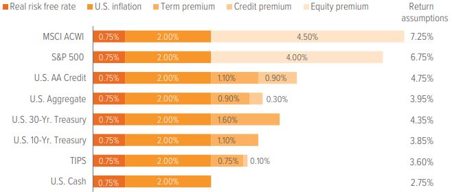
These forecasts use a building block methodology. Starting with our expectations for real short-term yield and inflation, we generate a risk-free rate forecast and, from that, derive all equity and fixed income assets by adding the relevant risk premium:

• We derive the risk premium for U.S. equities from the Gordon growth model, representing the sum of the dividend yield and the nominal earnings growth rate in excess of the risk-free rate. International equities forecasts add an international equity risk premium.
• Government bond return forecasts are the sum of the risk-free rate and an appropriate term premium. Corporate bond return forecasts add a credit risk premium.

From a theoretical perspective, all risk premiums mean-revert towards a long-run equilibrium, as the economy is in a steady state. The reason for mean reversion is that investment opportunities are time varying. Since the rate of arrival of new information is time varying, return volatility and covariance are time varying as well in the short run. Our econometric work and that of academic researchers confirms the stationarity of a number of risk premiums, which, in turn, justifies our assumption of constant average risk premiums, term premiums and credit spreads in the long-run equilibrium (Exhibit 5).

Exhibit 5. Long-run equilibrium return assumptions

As of 09/30/23. Source: Voya IM. Assumptions are subject to change.

Appendix: Methodological considerations

Covariance and correlation matrices methodology

Matrices of estimated asset class covariance and correlation are the underlying pillars of our asset class standard deviation forecasts. This is a different process than forecasting returns, as correlations tend to wander over time. If we were to use a historical average or exponentially weighted methodology—which takes a long-run history and puts a heavier weight on recent observations—it could lead to risk forecasts that may represent the past but bear little resemblance to the future. Therefore, the forecasted risk for asset classes is summarized by the return covariance matrix. These are crucial components of the capital market assumptions process.

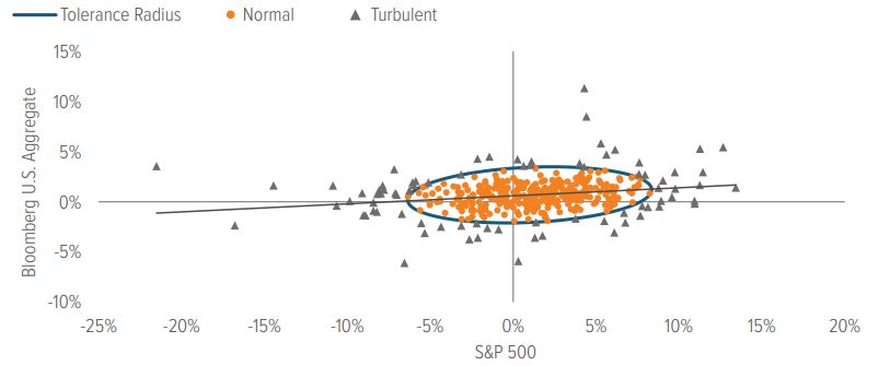
An example using stocks and bonds illustrates this point. Over the past 20 years, the correlation of returns between the S&P 500 Index and Bloomberg U.S. Aggregate Bond Index was -0.02; however, this offers little insight into the relationship between these two asset classes during unusual periods or when financial markets are in euphoric or pessimistic states. For example, over that same 20-year interval, the correlation of stocks to bonds was -0.10 during normal periods of returns but +0.07 during unusual periods (Exhibit 6). Incorporating these periods of unusual correlation patterns can lead to a truer estimate of the durability of diversification between asset classes. We capture these atypical periods in our standard deviation and correlation forecasts using an academic framework called turbulence.

Exhibit 6. It's critical to account for non-normal observations by taking into account correlations

Normal and turbulent periods of stock and bond correlations, 20 years ended 09/30/23

As of 09/30/23. Source: Voya IM.

Turbulence: Evolution from skulls to finance

The turbulence framework we use to estimate correlations and standard deviations of returns is derived from the academic work of the applied statistician Prasanta Chandra Mahalanobis. In the early 20th century, Mahalanobis analyzed human skull resemblances among castes and tribes in India. He created a formula to capture differences in skull size, which incorporated the standard deviation of measures of various skull parts. He then squared and summed the normalized differences, generating a single composite distance measure.³

This formula evolved into a statistical measure called the “Mahalanobis distance.” The measure was groundbreaking in that it helped analyze data across standard deviations but also incorporated the correlations among data sets. More than 70 years later, the Mahalanobis distance was used by Kritzman and Li to formulate a concept called "financial turbulence." ⁴ They postulated financial turbulence as a condition in which asset prices, given their historical patterns of returns, behave in an uncharacteristic way that including extreme price moves. They further noted that financial turbulence often coincides with excessive risk aversion, illiquidity and price declines for risky assets. We have used this turbulence framework (based on unusualness of returns and correlations of returns) to forecast risk measures in our capital market assumptions.

Observing turbulence

Turbulence can be calculated for any given set of asset classes. Back to our example of U.S. stocks and bonds, the two dimensions can be visualized as the equation of an ellipse using the returns of the S&P 500 Index and the Bloomberg U.S. Aggregate Index (Exhibit 6). The center of the ellipse represents the average of the joint returns of the two assets classes. The boundary is a level of tolerance that separates normal from turbulent observations. This boundary takes the form of an ellipse rather than a circle because it accounts for the covariance of the asset classes.

The idea captured by this measure is that certain periods are considered turbulent not only because returns are unusually high or low, but also because they moved in the opposite direction of what would have been expected based on the average correlation.

Using turbulence to create portfolios

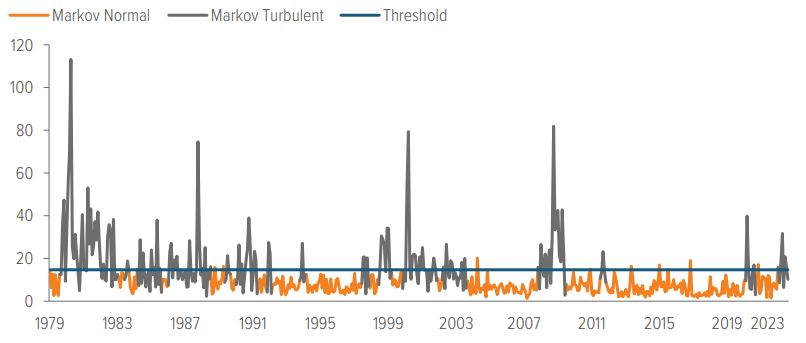
The threshold of normalcy and turbulence shown in Exhibit 6 is not static; rather, it changes over time. Our process identifies turbulent market regimes by estimating a covariance matrix covering those periods of market stress alone, using a Markov model. The model classifies regimes, rather than arbitrary thresholds, since thresholds would fail to capture the persistence of shifts in volatility (Exhibit 7).

Exhibit 7. Means and variances both matter when determining if observations are turbulent

Markov normal and turbulent regimes over time

As of 08/31/23. Source: Voya IM.

To identify turbulent market regimes, we make use of the concept of multivariate outliers in a return distribution. That is, we consider the deviation of a particular asset class’s return from the average, as well as its volatility and correlation with other asset classes. We subsequently estimate a covariance matrix based on periods of normal and turbulent market performance. Finally, we use a procedure to blend these two covariance matrices using weights to express views about the likelihood of each normal or turbulent regime and to capture the differential risk attitudes toward each. The weights we use to create our strategic asset allocation portfolios are 60% normal and 40% turbulent.

Although turbulent regimes have an observed frequency of only 30%, we overweight them at 40% to account for structural issues such as globalization, demographics and worldwide central bank intervention, which are prevalent today. Furthermore, overweighting turbulent periods increases the assumed risks, providing a more conservative matrix that emphasizes diversification during volatile periods. From this blended covariance matrix, we then extract the implied correlation matrix and standard deviations for each asset class. In our view, this process helps create a strategic asset allocation portfolio that can account for the empirical evidence that correlations will deviate through time.

Time dependency of asset returns and its impact on risk estimation

Recent research suggests that expected asset returns change over time in somewhat predictable ways, and that these changes tend to persist over long periods. Thus, changes among investment opportunities— all possible combinations of risk and return—are found to be persistent. This Appendix will set out the economic reasons for return predictability, its consequences for strategic asset allocation and the adjustments we have made to control for it in our estimation process.

In our view, the common source of predictability in financial asset returns is the business cycle. The business cycle itself is persistent, and this makes real economic growth predictable, to some extent. The fundamental reason for the business cycle’s persistence is that its components share the same qualities. Consumers, for example, tend to smooth consumption since they dislike abrupt changes in their lifestyles. Research on permanent income and lifecycle consumption provides the theoretical basis for consumers’ desire for a stable consumption path. When income is affected by transitory shocks, consumption should not change since consumers can use savings or borrowing to adjust consumption in well-functioning capital markets.

Robert Hall has formalized these ideas by showing that consumers will optimally choose to keep a stable path of consumption equal to a fraction of their present discounted value of human and financial wealth.⁵ Investment, the second component of GDP, is sticky, as corporate investment in projects is usually long term in nature. Finally, government expenditures also have a low level of variability. Over a medium-term horizon, negative serial correlation sets in, as the growth phase of the cycle is followed by a contraction, which subsequently is followed by renewed growth.⁶

"Empirical persistence of the business cycle makes financial asset returns somewhat predictable.

How does this predictability of economic variables affect the predictability of asset returns? Consider stocks as an example.

Equity values are determined as the discounted present value of future cash flows, and they depend on four factors: expected cash flows, expected market risk premium, expected market risk exposure and the term structure of interest rates.

• Cash flows and corporate earnings tend to move with the business cycle.
• The market risk premium is high at business cycle troughs, when consumers are trying to smooth consumption and are less willing to take risks with their income. It is low at business cycle peaks, when people are more willing to take risks. The market risk premium is a component of the discount rate in the present value calculation of the dividend discount model.
• A firm’s risk exposure (beta), another component of the discount rate, changes through time and is a function of its capital structure. Thus, a firm’s risk increases with leverage, which is related to the business cycle.
• The last component of the discount rate is the risk-free rate, which is determined by the term structure of interest rates. The term structure reflects expectations for real interest rates, real economic activity and inflation, which are connected to the business cycle.

Thus, equity returns, and financial asset returns in general, are predictable to a certain extent. Risk premiums of many assets tend to be high in bad macroeconomic times and low in good times.

This predictability of returns manifests itself statistically through autocorrelation. Autocorrelation in time series of returns describes the correlation between values of a return process at different points in time. Autocorrelation can be positive when high returns tend to be followed by high returns, implying momentum in the market. Conversely, negative autocorrelation occurs when high returns tend to be followed by low returns, implying mean reversion. In either case, autocorrelation describes dependence in returns over time.

Traditional mean-variance analysis focused on short-term expected return and risk assumes that returns do not exhibit time dependence and that prices follow a random walk. In a random walk, expected returns are constant, exhibiting zero autocorrelation; realized short-term returns are unpredictable. Volatilities and cross-correlations among assets are independent of the investment horizon. Thus, the annualized volatility estimated from monthly return data, scaled by the square root of 12, should be equal to the volatility estimated from quarterly return data, scaled by the square root of 4.

In the presence of autocorrelation, the scaling rule described above (using the square root of time) is invalid since the sample standard deviation estimator is biased and the sign of autocorrelation matters for its impact on volatility and correlations. Positive autocorrelation leads to an underestimation of true volatility. A similar result holds for the cross-correlation matrix bias when returns exhibit autocorrelation. As a result, the risk/return tradeoff can be very different for long versus short investment horizons.

In a multi-asset portfolio, in which different asset classes display varying degrees of autocorrelation, failure to correct for the bias of volatilities and correlations will lead to suboptimal mean variance-optimized portfolios in which asset classes that appear to have low volatilities receive excessive allocations. Such asset classes include hedge funds, emerging market equities and non–public market assets, such as private equity and private real estate, among others.

There are at least two ways to correct for autocorrelation:

• A direct method that adjusts the sample estimators of volatility, correlation and all higher moments.
• An indirect method that cleans the data first, allowing us to subsequently estimate the moments of the distribution using standard estimators.

"Removing return autocorrelation prevents underestimation volatility

Given that the direct methods become quite complex beyond the first two moments, our choice is to follow the second method and clean the return data of autocorrelation. Before we do that, we estimate and test the statistical significance of autocorrelation in our data series.

We estimate first-order autocorrelation as the regression slope of a first-order autoregressive process. We use monthly return data for the period 1979–2014. We subsequently test the statistical significance of the estimated parameter using the Ljung-Box Q-statistic.⁷ The Q-statistic is a statistical test for serial correlation at any number of lags. It is distributed as a chi-square with k degrees of freedom, where k is the number of lags. Here, we test for first order serial correlation, thus k = 1. About 80% of our return series exhibit positive and statistically significant first-order serial correlation based on associated p-values at the 10% level of significance.⁸

Khandani and Lo provide empirical evidence that positive return autocorrelation is a measure of illiquidity exhibited among a broad set of financial assets, including small cap stocks, corporate bonds, mortgage-backed securities and emerging market investments.⁹ The theoretical basis is that in a frictionless market, any predictability in asset returns can be immediately exploited, thus eliminating such predictability. While other measures of illiquidity exist, autocorrelation is the only measure that applies to both publicly and privately traded securities and requires only returns to compute.

Since the vast majority of the return series we estimate exhibits autocorrelation, we apply the Geltner unsmoothing process to all series. This process corrects the return series for first-order serial correlation by subtracting the product of the autocorrelation coefficient ρ and the previous period’s return from the current period’s return, then dividing by 1-ρ. This transformation has no impact on the arithmetic return, but the geometric mean is impacted since it depends on volatility. Thus, this correction is important for long horizon asset allocation portfolios.

Accounting for climate change

The majority of research concludes climate change is a significant risk to our planet’s ecosystem and, according to the International Monetary Fund (IMF) and many other well-respected institutions, is set to have major economic impacts on many countries.¹⁰ While we believe global economic outcomes will continue to be dominated by the business cycle and event stresses, climate change is a material issue, and its importance could increase going forward. Therefore, we believe climate change risks―both physical and transition¹¹―should be considered when making forecasts of the future. Physical risks, for the most part, are best incorporated at the security level, although there are certain countries and asset classes (e.g., real estate) for which it is easier to make a clear, broad connection.

There are a few channels through which climate change could theoretically influence capital market assumptions: macro, fundamentals and repricing.

Macro: Climate-related considerations impact consumer behavior, investment needs, financing, supply chain organization, cross-border trade and stranded assets. These are mostly transition-risk related, driven by government policy and market forces. Climate change’s effect on these variables flows directly to GDP growth and inflation, the magnitude of which will be partly driven by the increase in productivity enabling technologies.

Fundamentals: Top-line output establishes the base for what companies can earn. Profit margins form the other component of the equation. The transition is certain to affect industries to different degrees, but the consequences are difficult to forecast in aggregate, so we retain our tried-and-true approach of assuming profit margins mean-revert to equilibrium.

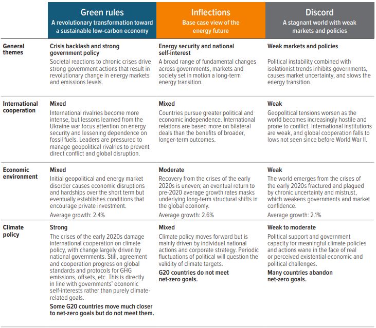
Repricing: Changes in valuation are the most difficult to gauge. Determinants of valuation at any one point and across time are highly uncertain, especially for broad asset classes (e.g., U.S. large cap equities), which is the level at which we forecast CMAs. We acknowledge that certain sectors generally deserve higher valuations than others and subscribe to the idea that capital will flow to more “sustainable” investments over time, but we argue that it is difficult to predict changes in relative pricing across sectors based on inherent “greenness,” especially across countries. Instead of comparing asset class carbon footprints based on sector compositions, we think sustainability characteristics should be defined at or below the industry level. Therefore, premiums and discounts for those factors, including climate change, should be applied to individual companies within their respective groups. As a result, our efforts are centered on macro and (to a lesser degree) fundamental inputs. To define and evaluate the impact of changes in climate related macro and fundamental inputs, we leaned on our partner (S&P Global) to develop plausible climate scenarios and expected economic outcomes. Although countless climate scenarios are plausible and investors would be well-served to stresstest portfolios against some of those possibilities, only one will occur. Therefore, we took the most likely climate scenario, called “Inflections” in Exhibit 8A, and integrated those assumptions into the global economic model for the base and alternative scenarios that form the backbone of our CMA.

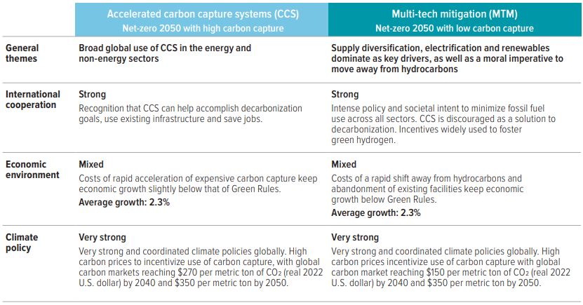
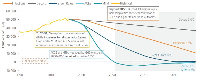
The climate scenarios (Exhibits 8A and 8B) are updated annually and developed within the context of achieving net-zero carbon emissions by 2050. This places them on a different time horizon than the economic scenarios used for our 10-year CMA, so they need to be rescaled, but these scenarios enable us to capture important developments along various temperature pathways.

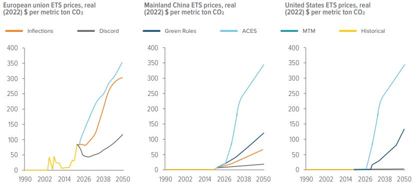
Unfortunately, given the lack of legally binding climate commitments by countries, daunting technological gaps and recent geopolitical strains, the current trajectory suggests a 2.4° Celsius increase in global average temperatures above preindustrial levels by 2100 (Exhibit 9). In this base-case scenario, the energy transition delivers fundamental change, with global emissions falling 25% from 2022 levels back to early 2000s readings, but geopolitical relations and diverging country trends based on national self-interest are likely to force adaptation rather than facilitate the necessary international cooperation. In all cases, a critical variable influencing emission paths is the price of carbon emissions and the government taxation, regulation and international coordination around it (Exhibit 10). To get to zero, emitting greenhouse gases (GHG) must become expensive relative to alternative means of production.

Like climate change itself, the impact on the economy is one that will be felt gradually. The difference in economic outcomes among most climate scenarios tested over the full horizon was modest. Thus, the impact of considering climate change in our capital market assumptions is minor. The exception, however, is the “Discord” scenario, in which countries become more inwardly focused, climate policies are inconsistent and decarbonization efforts lose momentum, resulting in limited meaningful action. In this case, global growth takes a sizable hit.

Over the 10-year forecast horizon, the economic damage would be mostly due to the series of crises that underlie the geopolitical rancor preventing climate change mitigation, as opposed to the negative effects of climate change itself. As the time horizon extends, however, so too does the risk of major and potentially irreversible physical costs.

What is clear from our analysis is that striving to address this negative externality will lead to an improved outlook for growth and for most risk assets, relative to taking no action. Moreover, incorporating views on climate change into our forecasts provides us with a more comprehensive picture of the world, which will help us generate better estimates going forward.

Exhibit 8A. Summary of base, optimistic and pessimistic climate scenarios

As of 09/23. Source: S&P Global. Forecasts are subject to change.

Exhibit 8B. Summary of net-zero climate scenarios

As of 09/23. Source: S&P Global. Forecasts are subject to change.

Exhibit 9. The path to 2050 and beyond: Emission trends and implied temperatures

Only the back-cast net-zero cases achieve the net-zero target of the Paris Agreement

As of 07/23. Source: S&P Global Commodity Insights. Forecasts are subject to change. Note: MtCO2 e=million metric tons of CO2 equivalent.

Exhibit 10. Lower-carbon outlooks see emission trading systems expand and prices rise

Net-zero cases assume global convergence of carbon pricing by 2050

As of 07/23. Source: S&P Global Commodity Insights. Forecasts are subject to change. ETS=emission trading system.

Multi-Asset Strategies and Solutions

Voya Investment Management’s Multi-Asset Strategies and Solutions (MASS) team, led by Chief Investment Officer Barbara Reinhard, manages the firm’s suite of multi-asset solutions designed to help investors achieve their longterm objectives. The team consists of 17 investment professionals who have deep expertise in asset allocation, manager research and selection, quantitative analysis and portfolio implementation. Barbara also leads the asset allocation team, which is responsible for constructing strategic asset allocations based on its long-term views. The team also employs a tactical asset allocation approach, driven by market fundamentals, valuation and sentiment, which is designed to capture market anomalies and reduce portfolio risk.

Download PDF

3228491   
1 S&P Global is an independent research firm that provides a comprehensive global macroeconomic model, linking 68 individual country models with key global drivers of performance. The model accounts for 95% of global GDP, covering 250–500 time series per country. 
2 “Understanding Glide Path Design: Distribution of Labor Income among Participant Populations,” Sinha, A. and Yuen, R., Voya Investment Management, 2Q18. 
3 Mahalanobis, P., “On the Generalized Distance in Statistics,” Proceedings of the National Institute of Sciences of India vol. 2 no. 1 (1936): 49–55. 
4 Kritzman, M. and Y. Li, “Skulls, Financial Turbulence, and Risk Management,” vol. 66 no. 5 (2010): 30–41. 
5 Hall, R., “Stochastic Implications of the Life-Cycle-Permanent Income Hypothesis: Theory and Evidence,” Journal of Political Economy 86 (1978): 971–988. 
6 Poterba, J. and Summers, L., “Mean Reversion in Stock Prices: Evidence and Implications,” Journal of Financial Economics 22 (1988): 27–60. 
7 Ljung, G.M. and Box, G.E.P., “On a Measure of Lack of Fit in Time Series Models,” Biometrika, 65, (1978): 297–303. 
8 The p-value is the probability of rejecting the null hypothesis of no serial correlation when it is true (i.e., concluding that there is serial correlation in the data when in fact serial correlation does not exist). We set critical values at 10% and thus reject the null hypothesis of no serial correlation for p-values <10%. 
9 Khandani, A.E. and Lo, A., “Illiquidity Premia in Asset Returns: An Empirical Analysis of Hedge Funds, Mutual Funds, and US Equity Portfolios,” Quarterly Journal of Finance 1 (2011): 205–264. 
10 International Monetary Fund, https://www.imf.org/en/Topics/climate-change/climate-and-the-economy#publications, accessed 10/31/22. 
11 Climate change risks can be divided into two categories: 1) physical risks, which result from climatic events such as wildfires, storms and floods; and 2) transition risks, which result from policy actions taken to shift the economy away from fossil fuels.

Past performance does not guarantee future results. This commentary has been prepared by Voya Investment Management for informational purposes. Nothing contained herein should be construed as (i) an offer to sell or solicitation of an offer to buy any security or (ii) a recommendation as to the advisability of investing in, purchasing or selling any security. Any opinions expressed herein reflect our judgment and are subject to change. Certain of the statements contained herein are statements of future expectations and other forward-looking statements that are based on management’s current views and assumptions and involve known and unknown risks and uncertainties that could cause actual results, performance or events to differ materially from those expressed or implied in such statements. Actual results, performance or events may differ materially from those in such statements due to, without limitation, (1) general economic conditions, (2) performance of financial markets, (3) interest rate levels, (4) increasing levels of loan defaults, (5) changes in laws and regulations and (6) changes in the policies of governments and/or regulatory authorities. The opinions, views and information expressed in this commentary regarding holdings are subject to change without notice. The information provided regarding holdings is not a recommendation to buy or sell any security. Fund holdings are fluid and are subject to daily change based on market conditions and other factors. 

The distribution in the United Kingdom of this presentation and any other marketing materials relating to portfolio management services of the investment vehicle is being addressed to, or directed at, only the following persons: (i) persons having professional experience in matters relating to investments, who are “Investment Professionals” as defined in Article 19(5) of the Financial Services and Markets Act 2000 (Financial Promotion) Order 2005 (the “Financial Promotion Order”); (ii) persons falling within any of the categories of persons described in Article 49 (“High net worth companies, unincorporated associations etc.”) of the Financial Promotion Order; and (iii) any other person to whom it may otherwise lawfully be distributed in accordance with the Financial Promotion Order. The investment opportunities described in this presentation are available only to such persons; persons of any other description in the United Kingdom should not act or rely on the information in this presentation. 

The Capital Markets Authority and all other Regulatory Bodies in Kuwait assume no responsibility whatsoever for the contents of this presentation and do not approve the contents thereof or verify their validity or accuracy. The Capital Markets Authority and all other Regulatory Bodies in Kuwait assume no responsibility whatsoever for any damages that may result from relying on the contents of this presentation either wholly or partially. It is recommended to seek the advice of an Investment Advisor. 

Voya Investment Management does not carry on a business in a regulated activity in Hong Kong and is not licensed by the Securities and Futures Commission. This insight is issued for informational purposes only. It is not to be construed as an offer or solicitation for the purchase or sale of any financial instruments. It has not been reviewed by the Securities and Futures Commission. Voya Investment Management accepts no liability whatsoever for any direct, indirect or consequential loss arising from or in connection with any use of, or reliance on, this insight, which does not have any regard to the particular needs of any person. Voya Investment Management takes no responsibility whatsoever for any use, reliance or reference by persons other than the intended recipients of this insight. Any prices referred to herein are indicative only and dependent upon market conditions. Unless otherwise specified, investments are not bank deposits or other obligations of a bank, and the repayment of principal is not insured or guaranteed. They are subject to investment risks, including the possibility that the value of any investment—and income derived therefrom, if any—can increase, decrease, or in some cases be entirely lost, and investors may not get back the amount originally invested. The contents of this insight have not been reviewed by any regulatory authority in the countries in which it is distributed. 

The opinions and views herein do not take into account your individual circumstances, objectives or needs and are not intended to be recommendations of particular financial instruments or strategies to you. This insight does not identify all the risks (direct or indirect) or other considerations which might be material to you when entering any financial transaction. You are advised to exercise caution in relation to any information in this document. If you are in doubt about any of the contents of this insight, you should seek independent professional advice. In addition, please be advised that Voya Investment Management is a non-Canadian company. We are not registered as a dealer or adviser under Canadian securities legislation. We operate in the Provinces of Nova Scotia, Ontario and Manitoba based on the international adviser registration exemption provided in National Instrument 31-103. Accordingly, investors will have more limited rights and recourse than if the investment manager were registered under applicable Canadian securities laws.